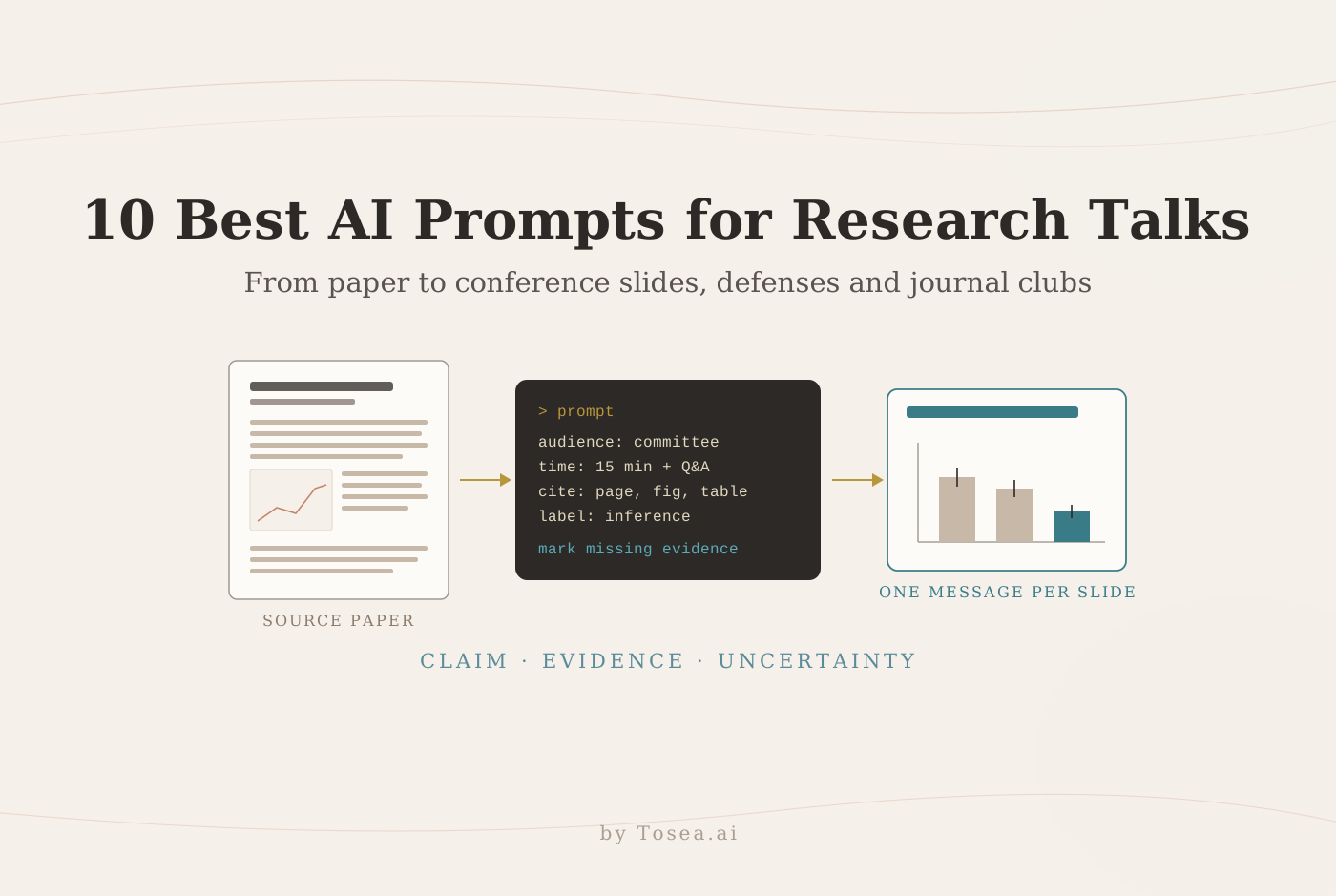
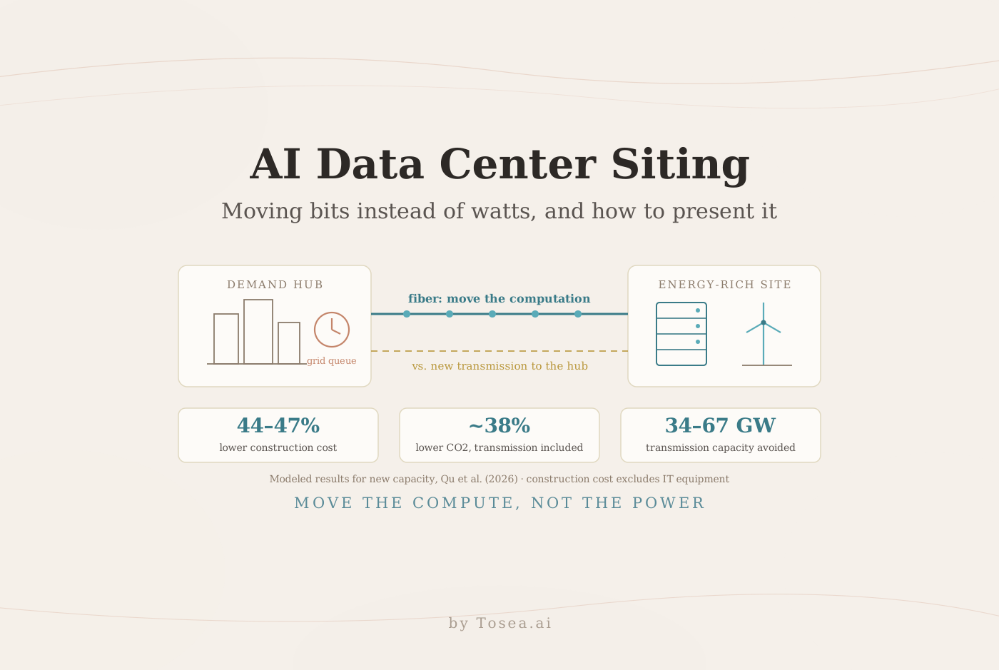
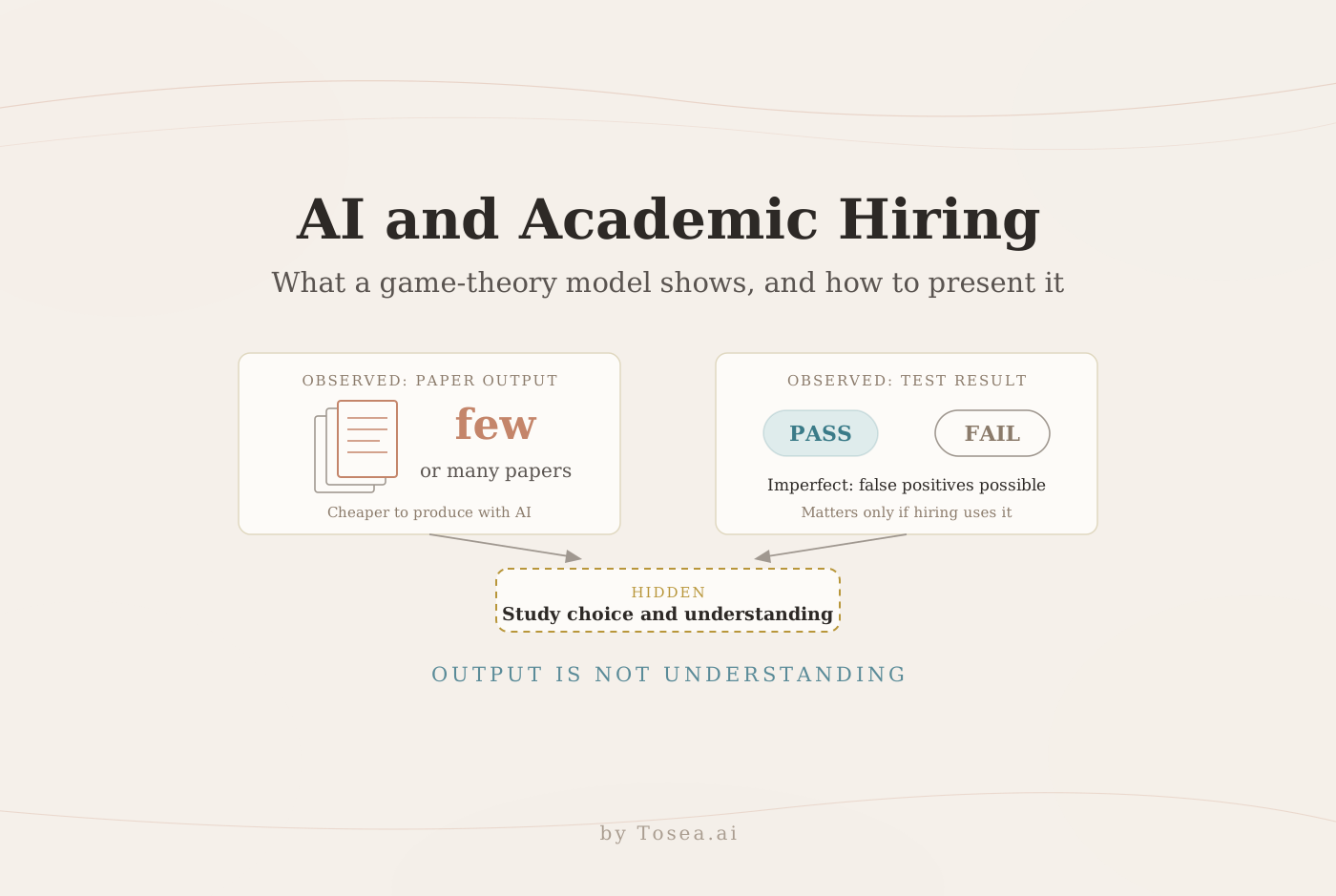
AI Ocean Forecasting: Why a Low RMSE Can Mislead and How to Present the Evidence
A new study tests Wenhai, Skyocean and ST-base on accuracy, physical consistency and fine-scale structure. What it found, what it cannot show, and four slides with AI prompts.
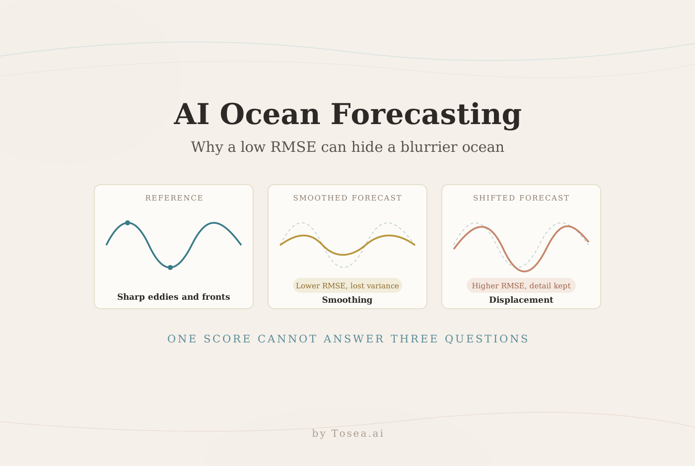
AI ocean forecasting can look better on a leaderboard while losing the eddies and fronts that make a forecast useful. A preprint posted on November 3, 2026 shows why: a smoother prediction can score well on pointwise error even when it suppresses fine-scale variation. Conversely, a forecast may retain a recognizable feature but place it slightly off target, and be penalized twice for it. That distinction matters when a team has to decide whether to improve feature placement, restore fine detail, or revisit the evaluation itself.
This guide explains what the study compared, what it found on each evaluation dimension, what it does not establish, and how to turn the evidence into four slides for a technical review.
What the study compared
Ziqing Zu, Ye Yuan, and colleagues propose three complementary ways to evaluate forecasts in A Multidimensional Evaluation Framework for Artificial Intelligence-Based Ocean State Forecasts (arXiv:2611.04892): overall pointwise accuracy, physical consistency, and distributional consistency. They compare Wenhai, Skyocean, and ST-base in a unified rolling forecast environment over the northwestern Pacific, from 10° to 35°N and 121° to 150°E. The test covers 120 daily initializations from January 1 through April 30, 2026 and forecast leads of one to seven days.
The systems retain their own inputs and configurations. Wenhai, for example, computes atmospheric forcing from atmospheric forecasts over the forecast period, while ST-base uses ocean and atmospheric analyses from the week before initialization. The comparison therefore concerns complete forecasting systems rather than the isolated effects of network architecture. The authors state that the objective is not to identify a universally best model.
The study at a glance
| Item | What the paper reports |
|---|---|
| Systems | Wenhai (global, 1/12°, up to 15-day leads), Skyocean (regional, 1/8°, up to 10 days), ST-base (regional, 1/12°, 50 levels, Swin Transformer baseline, up to 7 days) |
| Region | Northwestern Pacific, 10°–35°N, 121°–150°E |
| Period | 1 January to 30 April 2026, 120 daily initializations |
| Leads evaluated | Days 1–7; subsurface variables restricted to 0–644 m |
| Pointwise metrics | Bias, RMSE, and anomaly correlation in observation space (OceanPredict Class 4 approach) |
| Physical metrics | Stratification stability and geostrophic balance between sea surface height and surface currents |
| Distributional metrics | Tail RMSE with dynamic 10th/90th percentiles, power spectral density, scale-decomposed RMSE, neighborhood CRPS |
| References | OSTIA for sea surface temperature; AVISO L4 and SWOT L3 for sea level anomaly |
| Spatial scales | A: over 300 km; B: 70–300 km; C: under 70 km |
Pointwise accuracy asks how closely values match a reference at corresponding locations and times. Physical consistency asks whether variables agree with one another under selected physical diagnostics, using model outputs alone. Distributional consistency looks at extremes and how variance is distributed across scales. These questions need separate answers: a good score on one cannot compensate automatically for a failure on another.
What it found on each dimension
Pointwise accuracy depends on variable and lead time. For temperature, the Wenhai and Skyocean RMSE and anomaly correlation curves intersect after lead day 3; salinity shows a similar transition near day 6. ST-base temperature RMSE rises more steeply with lead time. All three forecasts show warm and saline biases.
Physical consistency can contradict a good pointwise score. Skyocean has relatively small pointwise sea level anomaly errors, yet its geostrophic balance residual falls only from about 0.176 m/s on day 1 to 0.138 m/s on day 7. Wenhai stays near 0.10 m/s and ST-base ranges from about 0.107 to 0.118 m/s.
Tails are harder than averages, and the reference matters. Extreme-event RMSEs are generally higher than full-sample RMSEs, and cold or low extremes generally have larger errors than warm or high extremes. For Skyocean, extreme-event sea level RMSE rises substantially when the reference changes from AVISO L4 to SWOT L3. That matters because AVISO L4 is used in Skyocean's training and inference, so SWOT acts as a more independent check.
Fine scales separate displacement from smoothing. At Scale C against SWOT L3, ST-base has a large RMSE but a small neighborhood CRPS and spectral amplitudes closer to SWOT, which suggests displacement. Skyocean has a smaller RMSE but a larger CRPS and a pronounced spectral deficit, which suggests smoothing and reduced variance.
Below are four original slide examples for a technical review. They illustrate how to present the evidence and are not screenshots from Tosea AI. Each prompt identifies the figure or section to use and tells the generator where to leave gaps instead of inventing data.
1. Replace the single winner slide with an evaluation plan
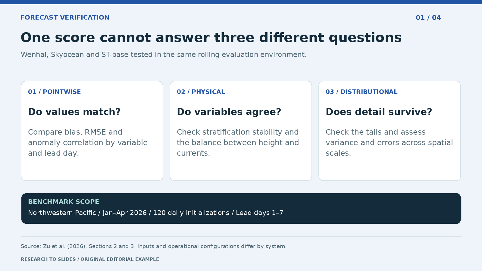
Figure 1. Editorial summary of the benchmark scope and three evaluation dimensions.
A model review should first ask which forecast behavior matters for the application. A team monitoring the large-scale background may focus on forecast-reference agreement by variable and lead day. A team studying fine structures needs evidence that the system preserves variability at the relevant scales. An audience concerned with physical interpretation also needs to know whether the forecast variables tell a coherent story.
Show the three dimensions on one slide, then give each its own evidence page. On a comparison chart, name the variable, depth where relevant, lead time, and reference product. Because the Wenhai and Skyocean temperature curves cross after day 3, a lead-averaged leaderboard would hide a change in relative performance that an operational user cares about.
Create one 16:9 benchmark overview using Sections 2 and 3. Show Wenhai, Skyocean, and ST-base, 120 daily initializations, January to April 2026, northwestern Pacific, and lead days 1 to 7. Use three columns: pointwise accuracy, physical consistency, and distributional consistency. State that inputs and configurations differ. Do not compute an aggregate ranking or invent scores.
2. Show the physical check next to the accuracy claim
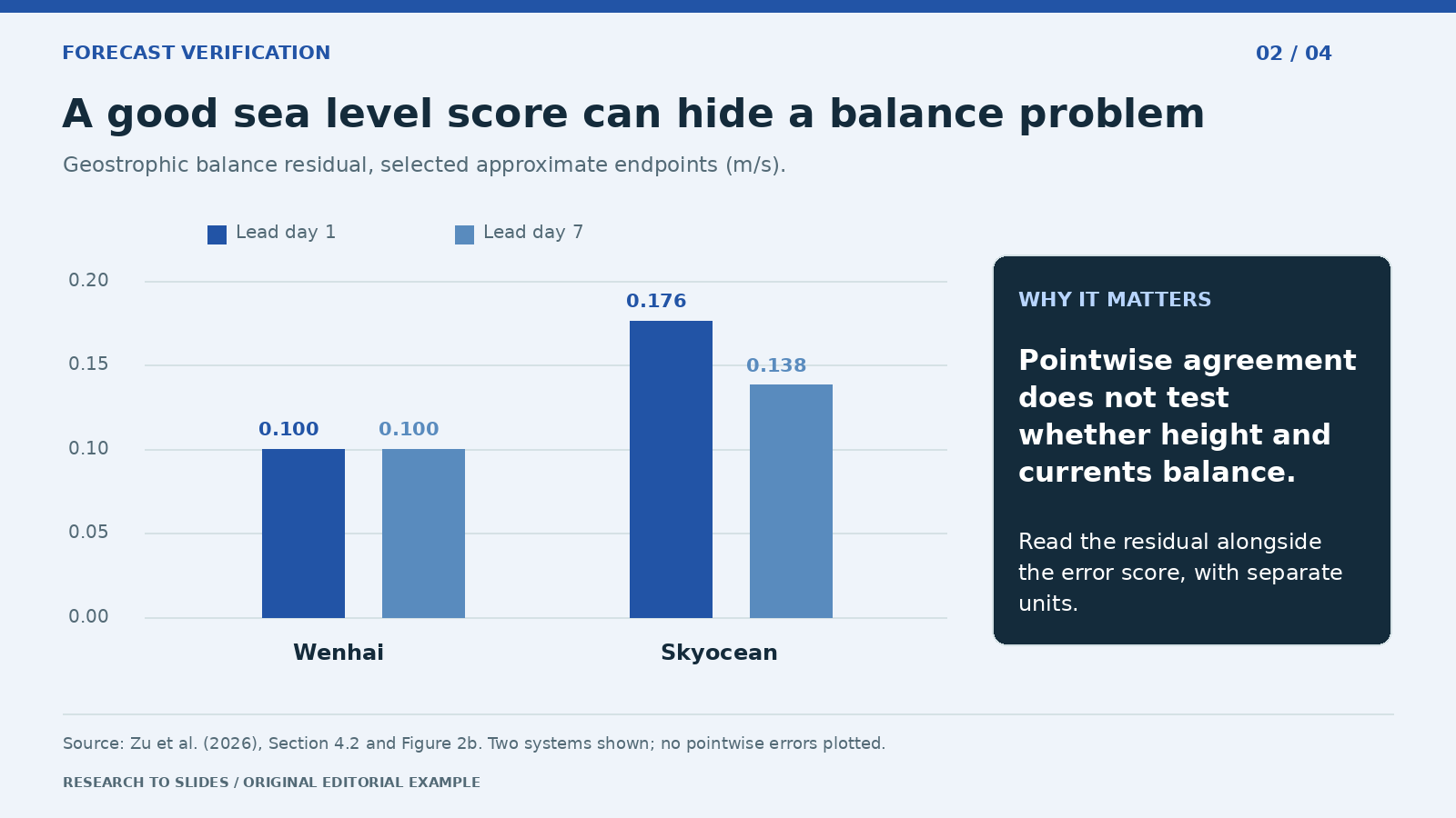
Figure 2. Approximate endpoints from Section 4.2 and Figure 2b, in meters per second. These bars show a balance residual, not pointwise sea level error. ST-base (about 0.107–0.118 m/s) is omitted for clarity.
A sea level anomaly forecast can agree relatively well with a reference while its height and current fields fit together less well. The residual measures how far surface currents depart from the currents implied by the sea surface height under geostrophic balance. The comparison is a useful way to explain why a cross-variable diagnostic can change the interpretation of an otherwise favorable score.
Do not place a sea level error and a velocity residual on the same numeric axis. Show them as separate evidence with distinct units and explain what each tests. The authors note that the residual is sensitive to the choice of deformation radius, filtering scale, and spatial weighting. It should not be presented as a complete check of ocean physics.
Create a one-slide physics check from Section 4.2. Plot approximate geostrophic balance residuals for Wenhai near 0.100 at days 1 and 7 and Skyocean 0.176 and 0.138. Start at zero and label units m/s. Note that these are selected endpoints and that ST-base ranged from about 0.107 to 0.118. Explain why low sea level anomaly error does not establish height-current coherence. Cite Figure 2b.
3. Show what average error misses in the tails
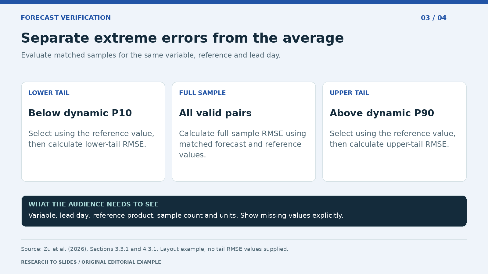
Figure 3. Reporting layout based on the study method. No unreported tail errors are supplied.
The average error does not tell an analyst how the system behaves during unusually warm or cold conditions. The paper separates lower- and upper-tail cases using dynamic thresholds built from 30 years of historical reference data: a linear trend is removed for each day of year and location, and the 10th and 90th percentiles are pooled over an 11-day window. Tail membership comes from the reference distribution, and errors are then calculated on those samples. Defining tails by the reference, rather than by the forecast, keeps events in the sample even when the model failed to predict them.
Show the full-sample score next to both tail scores for the same forecast variable and lead day. Keep the reference product visible, because the ranking can change with the reference. Do not add unreported confidence intervals or treat the 10th and 90th percentile cutoffs as warning thresholds.
Design a tail-error slide from Sections 3.3.1 and 4.3.1. Compare lower tail below the dynamic 10th percentile, all valid samples, and upper tail above the dynamic 90th percentile. Define tails using reference values. Include fields for variable, lead day, reference, sample count, and RMSE. Mark missing values as not supplied. Cite Figure 3 and avoid invented warning thresholds.
4. Diagnose the difference between a shifted feature and a smoothed one
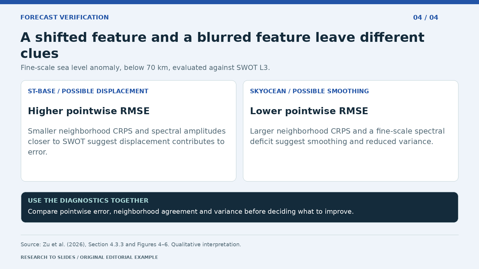
Figure 4. Qualitative synthesis for sea level anomaly at Scale C, below 70 km, evaluated against SWOT L3.
A forecast can place an eddy a little too far east and incur errors at both the observed and predicted locations. A different forecast can blur the eddy and reduce some pointwise errors while removing variation the user cares about. The distinction matters because improving spatial placement calls for different work than recovering lost structure.
The study combines scale-specific RMSE, neighborhood CRPS, and power spectral density. The first compares matched points, the second evaluates agreement with a local distribution and is less sensitive to small displacements, and the third shows where variance sits across wavelengths. The pattern for ST-base is consistent with displacement contributing to error; the pattern for Skyocean suggests smoothing and reduced variance. These are interpretations of multiple diagnostics, not diagnoses of every individual feature. See NASA's SWOT mission overview for context on the reference mission.
Create one 16:9 diagnostic slide for sea level anomaly against SWOT L3 at Scale C, below 70 km. Summarize the relative patterns for ST-base and Skyocean in RMSE, neighborhood CRPS, and spectral variance from Section 4.3.3. Label displacement and smoothing as suggested explanations. Add a reminder that reference resolution and sampling matter. Cite Figures 4 to 6; do not digitize or invent chart values.
What the study does not establish
The authors list the limits themselves, and a technical audience will ask about them. Put them on a slide rather than in the speaker notes.
- Scope. Three forecasting systems, one region, a four-month period, and lead times of 1–7 days.
- No overall winner. Rankings change with variable, lead time, reference, and scale.
- Metric sensitivity. The geostrophic balance metric depends on deformation radius, filtering, and weighting; spectral estimates near the grid scale depend on interpolation, sampling, and the reference's effective resolution.
- Missing physics. Daily-mean outputs without vertical velocity prevent checks of mass and potential vorticity conservation.
- System, not architecture. Different inputs and configurations mean results cannot be attributed to network design alone.
Five mistakes to avoid when presenting this paper
- Averaging across lead days. The temperature curves cross after day 3; a single number hides that.
- Mixing units on one axis. Sea level error in meters and a velocity residual in m/s belong on separate panels.
- Treating low RMSE as "best." In the authors' words, the forecast with the smallest pointwise sea level RMSE "exhibits a relatively large geostrophic imbalance and the greatest fine-scale variance deficit."
- Hiding the reference. Skyocean's extreme-event errors change substantially between AVISO L4 and SWOT L3.
- Digitizing figure values. Where the paper reports only curves, describe the pattern and cite the figure rather than reading numbers off a chart.
Tailor the same evidence to each audience
| Audience | Their question | Lead with | Keep visible |
|---|---|---|---|
| Operational forecasters | Which system should we trust at which lead? | Pointwise curves by variable and lead day | Curves cross; no aggregate ranking |
| Model developers | What should we fix? | Displacement versus smoothing diagnostics | Interpretation, not feature-level diagnosis |
| Evaluation or benchmark teams | How should we score models? | The three-dimension framework | Metric sensitivity and reference choice |
| Funders or managers | Is AI forecasting ready? | One slide per dimension with a plain-language takeaway | One region, four months, seven days |
For more on presenting technical charts so the evidence stays next to the claim, see our guides to building a data dashboard in PowerPoint and designing diagrams for presentations.
Build a research presentation in Tosea AI
Upload the paper to Tosea AI and ask for an outline with one claim, source, and intended decision per slide. Use the Layout and Diagram picker to choose a three-column overview, a two-panel comparison, or a diagnostic table before rendering. After generation, adjust the layout or diagram when the evidence is difficult to follow. Use a chart in HTML mode where the documented chart controls suit the supplied data.
Before exporting, verify the variable, units, lead time, reference, and whether each figure is schematic or quantitative. Check especially that no visual suggests a global ranking: the study spans three systems, one region, four months, and seven forecast leads. Layout Only is useful once the wording is approved, but the exported deck still needs an evidence check. For the general method of moving from a paper to slides, see the research paper to slides workflow, and for another infrastructure-research example, see how we presented AI data center siting research.
Q&A
Does a lower RMSE mean the ocean forecast is better?
It means the pointwise differences are smaller for the stated evaluation setup. Whether that makes the forecast better for a particular task also depends on physical consistency, tail performance, and the features the task needs to retain.
Why does the study use both AVISO L4 and SWOT L3?
AVISO L4 is a widely used gridded sea level product, but it is also used in Skyocean's training and inference. SWOT L3 provides an independent, higher-resolution reference. Comparing both helps show whether a low error is specific to one reference.
Can Tosea AI redesign my existing PowerPoint without changing the content?
Yes. Upload the PPTX or a PDF with Beautify PPT/PDF (available on Pro and above) and keep the default "Keep source pages" option, which preserves the page count, order, and content while redesigning the layout. Use Layout Only for later visual changes. Compare the result with the original, including labels, footnotes, and slide elements.
How do I upload a PowerPoint and ask Tosea AI to redesign each slide?
Upload the PPTX or PDF with Beautify, keep the source pages, and choose a template or describe the desired look. Inspect each redesigned slide before exporting.
Can I upload my own PowerPoint template to Tosea AI?
Yes, custom template upload is available on eligible paid plans. The custom template guide describes the Image mode workflow. Check the required layouts, fonts, colors, logo placement, and any master-slide rules in the output.
Can Tosea AI use custom brand colors, fonts, and a logo?
Yes. Specify approved colors and fonts, then supply a logo or custom template where supported by your plan. Verify font availability, color values, logo clear space, and contrast in PowerPoint.
Can Tosea AI match the style of my old company presentations?
Use a representative deck as design guidance. This does not mean the model is permanently trained on your style. For repeatable results, use an approved template and check the new slides against your organization's brand guidelines.
Does Tosea AI preserve PowerPoint formatting after export?
Editable PPTX export is designed to stay close to the preview while leaving supported elements editable. Complex graphics, fonts, and the viewing application can affect fidelity. Open the export in the PowerPoint environment where it will be presented.
Can I tell AI to edit the layout only and keep the exact wording?
Yes. Select Layout Only when the wording is already approved. After the edit, verify the text, labels, citations, footnotes, and line breaks against the source.
Give the audience a better question than who won
Use Tosea AI to turn the source paper into a deck that shows which metric answers which question. Choose the structure in the outline and adjust individual pages after rendering so the evidence stays next to the claim it supports. For more research-to-slides examples, see our guides to presenting AI risk disclosure research and presenting the BIS findings on AI and population ageing.
Sources
- A Multidimensional Evaluation Framework for Artificial Intelligence-Based Ocean State Forecasts — Ziqing Zu, Ye Yuan, et al., arXiv preprint, November 3, 2026
- Full paper PDF — arXiv (models in Section 2.1; configuration in Section 2.3; framework in Section 3; results in Section 4; limitations in Section 5.4)
- SWOT mission overview — NASA Science
- Layout and diagrams and Beautify an existing PPT or PDF — Tosea AI Help Center